SVM
SVM(Support Vector Machine)是一种模式识别(Pattern Recognition)的方法,可以作为分析数据进行处理的模型。主要是进行分类。
SVM用一系列的训练集(Train Set),建立一个特征参数的模型。所有的数据被标记为二个集合中的一个,如{是,不是}。然后通过测试集(Test Set)对训练好的模型进行评测。这一系列工作可以通过SVMTorch或者SVMLight完成。
VAD检测
现在可以看一下SVM简单的应用。在语音识别设备中,需要对语音信号的起始和终止做出划分,然后把这个语音信号送到下一级进行识别处理。这也就是VAD检测(Voice Activation Detection)。
现借用一个有180段录音的音频数据进行测试实验。音频数据里的内容是“天天”“华华”。采样率为16000bps。对信号分帧,256个点作为一帧(frame)。一帧数据获取到的语音特征过少,所以把10帧合成为一窗(window)进行特征提取。通过人工对这些windows进行标记,是语音窗标记为+1,作为正例。不是语音窗标记为-1,作为负例。
从所有windows中选取8000个正例和8000个负例形成trainset,剩下的windows作为testset。从上一步生成的“华华”和“天天”的cell中读取数据。Matlab代码如下:
    clear all;
    clc;
    close all;
    load xtrain_s_hh;
    total_length=0;
    x1=zeros(62000,451);

    for i=1:length(xtrain_s_hh)
        a=xtrain_s_hh{i};
        current_length=total_length;
        total_length=total_length+size(a,1);
        for j=1:size(a,1)
            x1(current_length+j,:)=xtrain_s_hh{i}(j,:);
        end
    end


    clear xtrain_s_hh; %防止Out of Memory
    load xtrain_s_tt;

    for i=1:100
        a=xtrain_s_tt{i};
        current_length=total_length;
        total_length=total_length+size(a,1);
        for j=1:size(a,1)
            x1(current_length+j,:)=xtrain_s_tt{i}(j,:);
        end
    end
    clear xtrain_s_tt;
然后进行trainset和testset的生成:
    loaddata;
    % trainset
    posSet = x1(x1(:, end)==1, :);
    negSet = x1(x1(:, end)==-1, :);

    aa = randperm(9933);
    trainSet = posSet(aa(1:8000), :);

    bb = randperm(52205);
    trainSet = [trainSet; negSet(bb(1:8000), :)];
    sum(trainSet(:, end)==-1)

    % testset
    testSet = posSet(aa(8001:end), :);
    testSet = [testSet; negSet(bb(8001:10000), :)];

    % transform 451 to 30 dimensions
    dimension=30;
    feature=3;
    xtrain_lab1=[];
    for gap=0:9
        temp=[trainSet(:,(13+gap*45):(15+gap*45))];
        xtrain_lab1=[xtrain_lab1,temp]; %30 dimensions
    end
    xtrain_lab1=[xtrain_lab1,trainSet(:,451)];

    xtest_lab1=[];
    for gap=0:9
        temp=[testSet(:,(13+gap*45):(15+gap*45))];
        xtest_lab1=[xtest_lab1,temp];
    end
    xtest_lab1=[xtest_lab1,testSet(:,451)];

    % "xtrain_lab1" normalization
    X = xtrain_lab1(:, 1:dimension)';
    y = X(:);
    Y = reshape(y, feature, size(xtrain_lab1, 1)*size(xtrain_lab1(:, 1:end-1), 2)/feature)';
    xtrain_norm = zeros(size(Y));
    MaxVec = max(Y, [], 1);
    MinVec = min(Y, [], 1);
    for idx = 1:feature
        x = Y(:, idx);
        lggr = x >= MaxVec(idx);
        lgle = x <= MinVec(idx);
        lgbe = x > MinVec(idx) & x < MaxVec(idx);
        x(lggr) = 1;
        x(lgle) = 0;
        x(lgbe) = (x(lgbe) - MinVec(idx)) / (MaxVec(idx) - MinVec(idx));
        xtrain_norm(:, idx) = x;
    end
    X = xtrain_norm';
    y = X(:);
    xtrain_norm_win = reshape(y, dimension, length(y)/dimension)';
    xtrain_norm_win = [xtrain_norm_win, xtrain_lab1(:, end)];

    % "xtest_lab1" normalization
    X = xtest_lab1(:, 1:dimension)';
    y = X(:);
    Y = reshape(y, feature, size(xtest_lab1, 1)*size(xtest_lab1(:, 1:end-1), 2)/feature)';
    xtest_norm = zeros(size(Y));
    for idx = 1:feature
        x = Y(:, idx);
        lggr = x >= MaxVec(idx);
        lgle = x <= MinVec(idx);
        lgbe = x > MinVec(idx) & x < MaxVec(idx);
        x(lggr) = 1;
        x(lgle) = 0;
        x(lgbe) = (x(lgbe) - MinVec(idx)) / (MaxVec(idx) - MinVec(idx));
        xtest_norm(:, idx) = x;
    end
    X = xtest_norm';
    y = X(:);
    xtest_norm_win = reshape(y, dimension, length(y)/dimension)';
    xtest_norm_win = [xtest_norm_win, xtest_lab1(:, end)];
这里选取能量,过零率,能量*过零率值,MFCC的12个特征值作为一个帧的特征,那么一个window的特征就是150维。这里先不进行PCA降维。然后将这些标记了+1,-1的特征进行输出,格式遵照SVMlight或者SVMtorch的格式要求。这里用SVMlight。
    fidTrain = fopen('xtrain_light_norm_30d.txt','w');
    fidTest = fopen('xtest_light_norm_30d.txt','w');
    for idx = 1:size(xtrain_norm_win, 1)
        one = xtrain_norm_win(idx, :);
        fprintf(fidTrain,'%+d ',int8(one(end)));
        for j = 1:(size(xtrain_norm_win,2)-1)
            fprintf(fidTrain,[int2str(j) ':%f '], one(j));
        end
        fprintf(fidTrain,'\n');
    end

    for idx = 1:size(xtest_norm_win, 1)
        one = xtest_norm_win(idx, :);
        fprintf(fidTest,'%+d ',int8(one(end)));
        for j = 1:(size(xtest_norm_win,2)-1)
            fprintf(fidTest,[int2str(j) ':%f '], one(j));
        end
        fprintf(fidTest,'\n');
    end
    fclose(fidTrain);
    fclose (fidTest);
接下来用testset测试出用不同参数调出的最优模型。
训练出的模型如何导入到实时程序进行判定
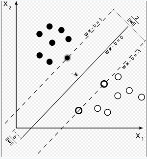
| 如图所示,Xi为特征向量,Yi为{-1,1}集合中的值。通过上面的训练找出最优的超平面 W•X-b=0,W为超平面的法向量。b/ | W | 是法向量的长。那么黑色的点满足W•Xi-b > 1,白色的点满足W•Xi-b < -1。那么在程序里就可以进行实时jugde了,步骤如下: |
- 用选定的trainset训练出model,model实质也就是W向量和b的值。打开SVMlight可以看见有多个支持向量和一个b值。
- 把Matlab算得的系数(W,b)以合适的形式(数组,结构体)放入到C中。
- 实时采样的语音信号通过C里的特征(MFCC,过零率,能量)提取程序算得指定维度的特征Xi。
- 通过计算W•Xi-b的值大于1或者小于-1得出采样信号是不是语音信号。
需要注意的是,Matlab的特征提取程序必须和C完全一致。不然训练出model的那些系数直接放到C里面就不适用了。
Train && Test
笔者采用SVMlight工具进行训练和测试。在svmlight软件目录下执行命令:
./svm_learn xtrain_150d.txt
训练结果如下:

然后对生成的模型svm_model_150d进行测试,执行命令
./svm_classify xtest_light_norm_150d.txt svm_model output_150d
得到如下结果:
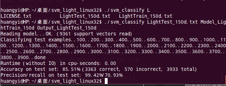
recall为71%左右,效果还算理想,后面应该对特征进行重新选择或者对训练的参数进行微调。
加入参数-c ./svm_classify -c 0.01 xtest_light_norm_150d.txt svm_model output_150d
Precision / Recall比率高达97.67% /90.95%,这就可以用这个模型进行C实现了。
模型进行参数转换
svm_light训练出来的模型数据格式是这样的:
SVM-light Version V6.02
150 # highest feature index
16000 # number of training documents
2467 # number of support vectors plus 1 2466 vectors
14.60996 # threshold b, each following line is a SV (starting with alpha*y)
-0.10000000000000000555111512312578 1:-2.6072149 2:-0.386718 3:-4.7835841 4:1.24163 5:-2.846272 6:2.602037 7:-2.354259 8:2.0891199 9:0.71786201 10:-0.762326 11:0.94002402 12:-0.43815601 13:0.013226 14:0 15:0 16:-4.1096439 17:-1.669122 18:-4.8028402 19:3.3105819 20:0.51009297 21:4.9304528 22:-4.73594 23:0.34844199 24:1.549247 25:0.031539001 26:2.0623391 27:-0.066358998 28:0.015391 29:0 30:0 31:-5.746675 32:-0.237827 33:0.197589 34:4.5699081 35:0.0037120001 36:2.6799929 37:-3.70121 38:-1.757226 39:-0.72618198 40:-2.49002 41:0.69152498 42:-0.457647 43:0.032465 44:0 45:0 46:-6.4179931 47:-0.69469702 48:-0.69478399 49:3.78141 50:0.31874901 51:-0.39264899 52:-3.5847859 53:1.812808 54:0.81401801 55:-2.5526011 56:-0.32375601 57:-0.69582701 58:0.090738997 59:0 60:0 61:-5.1000252 62:-2.146148 63:-4.458828 64:3.943033 65:-0.117736 66:1.385269 67:-4.1872921 68:0.50814003 69:0.365538 70:-0.013903 71:-0.178859 72:-0.49208501 73:0.029083 74:0 75:0 76:-7.209651 77:-3.5355501 78:-3.4768031 79:5.466105 80:0.90299797 81:2.5297711 82:-0.87344199 83:2.061152 84:-0.52099699 85:-0.489656 86:1.120425 87:-0.34177899 88:0.012507 89:0 90:0 91:-2.4900229 92:0.87366498 93:-1.219308 94:6.570838 95:-0.66704899 96:2.664654 97:-2.772584 98:2.3200381 99:0.128732 100:-1.34489 101:1.447106 102:-0.264539 103:0.016508 104:0 105:0 106:-3.7242949 107:1.571139 108:0.61830097 109:5.7569218 110:0.104916 111:-0.21683399 112:-3.0075519 113:1.499946 114:-0.30457601 115:-0.90873897 116:1.7306581 117:-0.101519 118:0.015194 119:0 120:0 121:-3.0614409 122:-0.53184998 123:-3.157887 124:4.1598859 125:-2.2302539 126:2.255312 127:-3.982137 128:0.69850898 129:0.98338699 130:-0.70040601 131:0.25580299 132:-0.40691599 133:0.021459 134:0 135:0 136:-3.491164 137:1.186574 138:-1.103568 139:3.5958719 140:2.343365 141:4.7770991 142:0.943187 143:1.168201 144:-0.040600002 145:1.175315 146:1.391314 147:-0.060185999 148:0.018883999 149:0 150:0 #
现在把这些系数转为C语言能处理的数组形式,采用python进行处理。
    #! /usr/bin/python
    # -*- coding: utf8 -*-
    f = open("model")
    out = open("coff.txt",'w')
    lines = f.readlines()
    f.close

    l_list = lines[11:]  #从第12行开始
    for l in l_list:
    	    for ele in l.strip().split(' '):
		    if ':' in ele:
			    kv=ele.split(':')
		            k=kv[0]
			    v=kv[1]
			    out.write(v+',')
处理后的数据格式就是
-2.6072149,-0.386718,-4.7835841,1.24163,-2.846272,2.602037,-2.354259,2.0891199, 0.71786201,-0.762326,0.94002402,-0.43815601,0.013226,0,0,-4.1096439,-1.669122, -4.8028402,3.3105819,0.51009297,4.9304528,-4.73594,0.34844199,1.549247,0.031539001, 2.0623391,-0.066358998,0.015391,0,0,-5.746675,-0.237827,0.197589,4.5699081,0.0037120001, 2.6799929,-3.70121,-1.757226,-0.72618198,-2.49002,0.69152498,-0.457647,0.032465,0,0, -6.4179931,-0.69469702,-0.69478399,3.78141,0.31874901
写为二维数组可以这样,
double SVMCoff[M][N]={-2.6072149,-0.386718,-4.7835841,1.24163,-2.846272,2.602037, -2.354259,2.0891199,0.71786201,-0.762326,0.94002402,-0.43815601,0.013226,0,0, -4.1096439,-1.669122,-4.8028402,3.3105819,0.51009297,4.9304528,-4.73594,0.34844199, 1.549247,0.031539001,2.0623391,-0.066358998,0.015391,0,0,-5.746675,-0.237827,0.197589, 4.5699081,0.0037120001,2.6799929,-3.70121,-1.757226,-0.72618198,-2.49002,0.69152498, -0.457647,0.032465,0,0,-6.4179931,-0.69469702,-0.69478399,3.78141,0.31874901};
用Matlab解析模型文件
实际上,上面用python读取模型文件中的数据转为二维数组是没有必要的。记在这里作为一种方法积累。因为在前面的时候还不知道模型里面那么多的支持向量到底应该怎么进行应用,直到我开启了Matlab.
    clear all
    modelfl = fopen('Model_LightTrain_150d_1','r');
    version_buffer = fscanf(modelfl,'SVM-light Version %s\n');
    kernel_type = fscanf(modelfl,'%d # kernel type\n', 1);
    poly_degree = fscanf(modelfl,'%d # kernel parameter -d \n', 1);
    rbf_gamma = fscanf(modelfl,'%f # kernel parameter -g \n', 1);
    coef_lin = fscanf(modelfl,'%f # kernel parameter -s \n', 1);
    coef_const = fscanf(modelfl,'%f # kernel parameter -r \n',1);
    parm_custom = fscanf(modelfl,'%s kernel parameter -u \n',1);
    total_words = fscanf(modelfl,'%d # highest feature index \n',1);
    total_doc = fscanf(modelfl,'%d # number of training documents \n',1);
    sv_num = fscanf(modelfl,'%d # number of support vectors plus 1 \n',1);
    thresh_b = fscanf(modelfl,'%f # threshold b, each following line is a SV (starting with alpha*y)\n',1);
    sv_num = sv_num - 1;
    alpha = zeros(sv_num, 1);
    weight_sv = zeros(sv_num, total_words);
    for i=1:sv_num
        alpha(i,1) = fscanf(modelfl,'%f ',1);
        for k=1:total_words-1
            str_format = sprintf('%d:%%f ',k);
            weight_sv(i,k) = fscanf(modelfl,str_format,1);
        end
        str_format = sprintf('%d:%%f #\n',total_words);
        weight_sv(i,total_words) = fscanf(modelfl,str_format,1);
    end
    fclose(modelfl);% Linear Weight Support Vectors
    for i=1:sv_num
        for k=1:total_words
            weight_sv(i,k) = alpha(i)*weight_sv(i,k);
    end
    end
    lin_weight = sum(weight_sv,1);

    % verify the output
    modelf2 = fopen('LightTest_150d.txt','r');
    sv_num=10;
    for i=1:sv_num
        alpha2(1,1) = fscanf(modelf2,'+%d ',1);
        for k=1:150
            str_format2 = sprintf('%d:%%f ',k);
            weight_sv2(i,k) = fscanf(modelf2,str_format2,1);
        end
    end
    fclose(modelfl);% Linear Weight Support Vectors

    for i=1:10
        out(i,:)=weight_sv2(i,:).*lin_weight;
    end
    All=sum(out,2);
    All=All-thresh_b;
后面一段代码verify the output是从测试集里取10个数据和svm_classify生成的结果对比来验证以上算法的正确性。实验结果完全一样。
那么就可以得出模型文件的正确用法了.
- 首先是weight_sv(i,k) = alpha(i)*weight_sv(i,k),用每一个支持向量乘以每行开头的alpha获得权重。
- 然后lin_weight = sum(weight_sv,1),每一列相加。这样不管是多少个支持向量,最终得到的是一个150*1的矩阵,即150个系数。
- 这150个系数和一窗语音算出的150个特征点乘后累加。
- 累加后的值减去thresh_b和+1 -1作比较就可以得出判断是否是语音段了。
References
[1].http://www.cs.cornell.edu/People/tj/svm_light/
[2].http://en.wikipedia.org/wiki/Support_vector_machine
[3].http://blog.csdn.net/carpinter/article/details/7375309